Perceptron

Weight Sparsity vs Data Sparsity

MoE layers achieve efficiency through weight sparsity: each token activates only k of N experts. But this is only half the story.

Think of routing as a matrix R where columns are experts and rows are tokens. Weight sparsity constrains the rows – each token uses at most k experts. Data sparsity constrains the columns – each expert processes a bounded number of tokens.

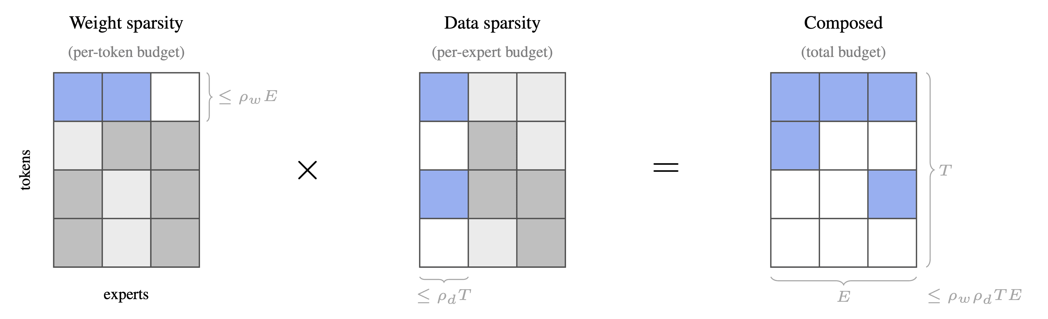
These are orthogonal. Weight sparsity asks "which experts for this token?" Data sparsity asks "which tokens for this expert?" Composing both gives you a budget over the full matrix.

Why does this matter? Not all tokens need equal compute. Blank image patches, punctuation, predictable continuations – these don't deserve the same budget as dense, information-rich tokens. Data sparsity lets the model skip compute where it's not needed.

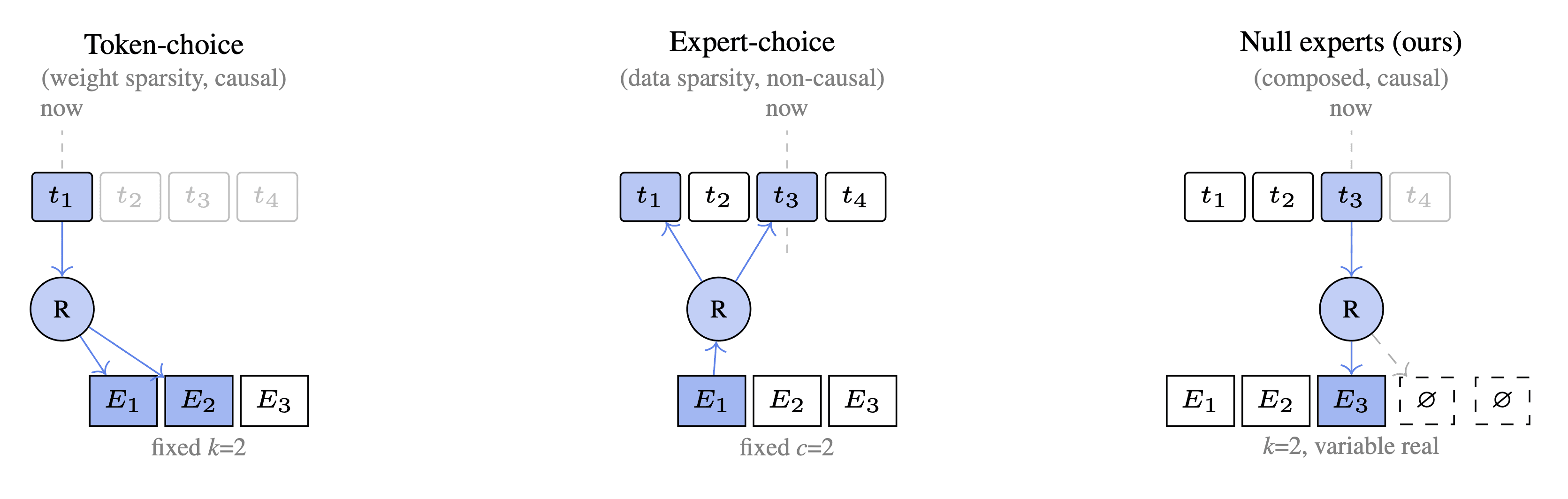
The challenge: expert-choice routing implements data sparsity naturally (experts pick their tokens), but it requires seeing future tokens – violating causality for autoregressive models. Token-choice routing is causal but assigns exactly k experts to every token.

We want both: token-choice causality with variable compute per token.

Implementation: Null Experts

We add "null experts" to the routing pool – experts that output zero. When a token routes to null experts, those slots skip computation. Standard load balancing over the expanded pool (real + null experts) encourages data sparsity in expectation.

The implementation is a few-line change on top of standard token-choice MoE. Highlighted lines show the diff from standard token-choice MoE:

Token-Choice MoE with Null Experts
──────────────────────────────────

Input: x (T, D), router weights W (N+1, D), experts E, top-K, null copies M

# Router
logits = x @ W.T                                          # (T, N+1)
logits = cat([logits[:, :N], logits[:, N:].expand(M)])   # (T, N+M)  ← ADDED
scores = softmax(logits)
top_scores, top_idx = top-K(scores, k)

# Reorder tokens by expert
order = argsort(top_idx.flatten(), stable=True)
sorted_scores = top_scores.flatten()[order]
sorted_tokens = order // k
num_per_expert = histc(top_idx, bins=N+M)                #           ← CHANGED

# Truncate to real experts (null experts sort last)
num_real = num_per_expert[:N].sum()                      #           ← ADDED
sorted_scores[:num_real] /= per_token_sum(...)           # renorm    ← ADDED

# Expert computation (unchanged grouped_mm)
x_in = x[sorted_tokens[:num_real]] * sorted_scores[:num_real, None]
x_out = grouped_mm(x_in, E, num_per_expert[:N])          #           ← CHANGED

# Scatter back
y = zeros(T, D)
y.scatter_add_(sorted_tokens[:num_real], x_out)
return y

The key insight: argsort places null expert indices at the end, so we just slice [:num_real] and run the same grouped matmul. The kernel is unchanged – it already handles variable tokens-per-expert.

To target data sparsity ρ with N real experts, we use M = N·(1-ρ)/ρ null copies. At N=64: ρ=0.5 needs M=64 copies; ρ=0.25 needs M=192.

Results

We train vision-language models upcycling to MoEs from two base model scales - Qwen3 0.6b and 1.7b - varying data sparsity while controlling expected compute.

Our notation:

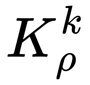
means top-k routing at sparsity ρ, so expected real experts = k·ρ.

Scaling Data Sparsity

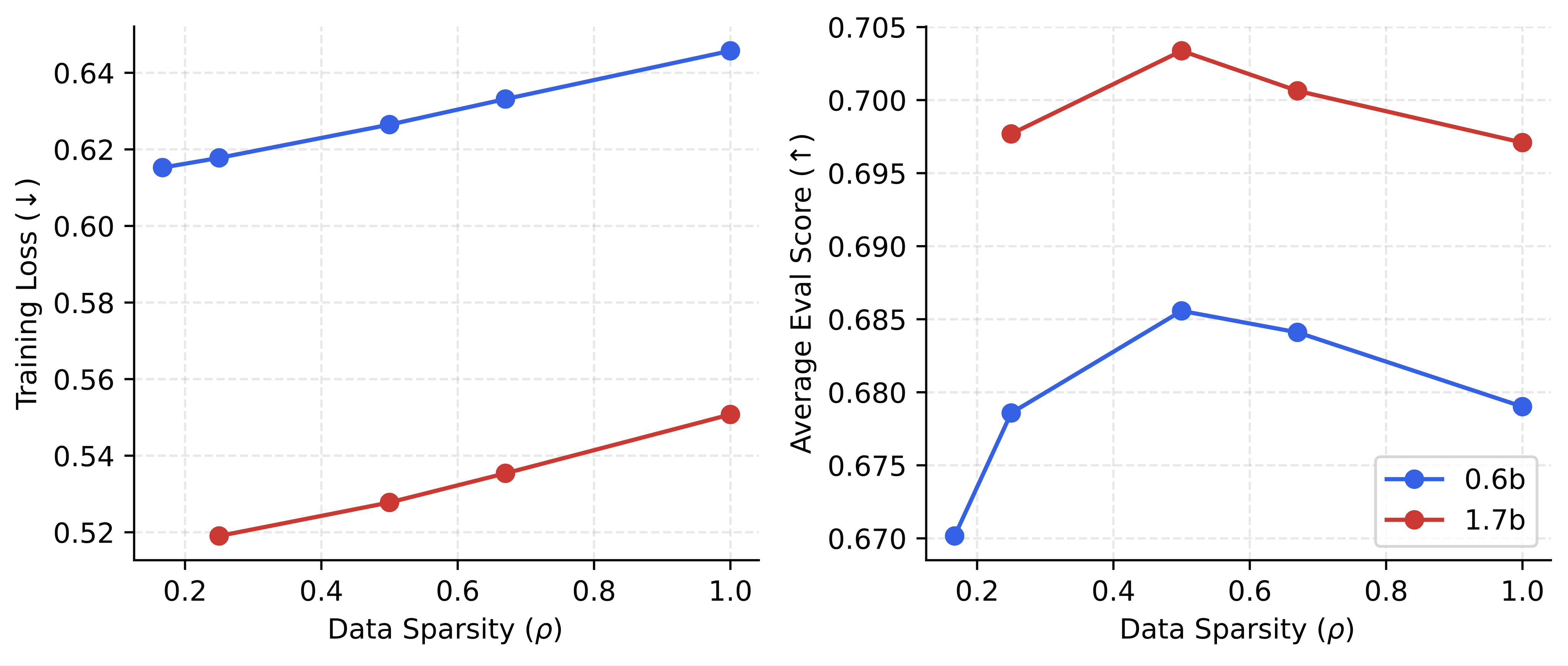
At fixed expected compute (E[K]=2), we vary sparsity from ρ=1.0 (dense) to ρ=0.17.

Training loss improves monotonically with sparsity – confirming that sparser configurations can always recover denser solutions (the solution space is preserved). Evaluation peaks around ρ≈0.5, then degrades at aggressive sparsity. We restrict subsequent experiments to ρ≥0.5.

Compute Efficiency

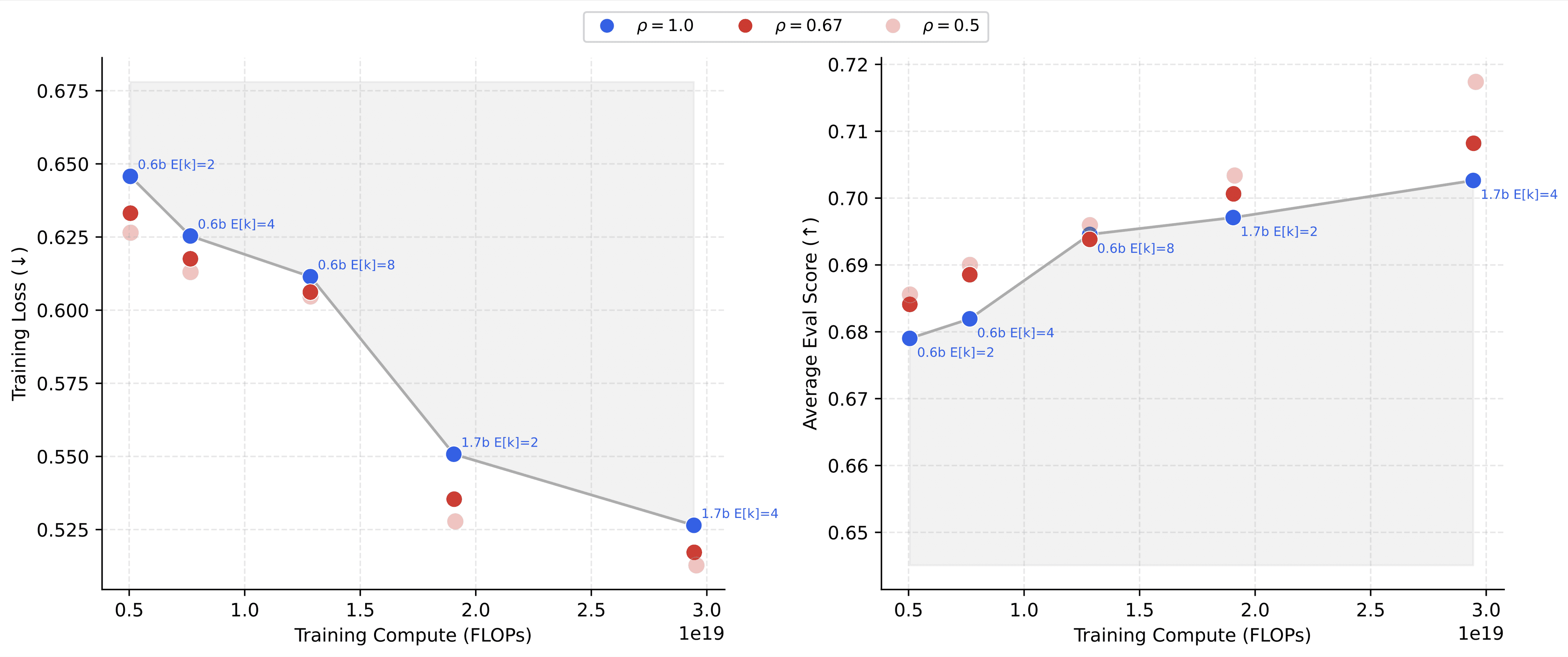
Across model scales and compute budgets, data-sparse configurations (red) consistently outperform data-dense baselines (blue) at matched expected FLOPs. Data sparsity reveals a better Pareto frontier.

Extended Training

Task Benchmark	1.7B K⁴_1.0 18B-A3B	1.7B K⁸_0.5 18B-A3B	Isaac 0.2 2B	InternVL3.5-20B-A4B 20B–A4B
Pointing
Pointing — Aerial Grounding	80.7	82.2	73.1	—
Pointing — Perceptron Grounding	58.8	59.2	51.5	—
Pointing — RefCOCO	87.6	87.8	87.4	91.9
Pointing — Overall	75.7	76.4	70.7	—
OCR
OCR — ChartQA	79.0	80.3	75.1	86.6
OCR — DocVQA	92.9	93.8	92.1	92.9
OCR — A-OKVQA (val)	89.4	91.8	87.2	—
OCR — TextVQA	80.8	82.0	78.1	78.5
OCR — OCRBench	873	880	857	870
OCR — Overall	85.9	87.2	83.6	—
Counting
Counting — Aerial Counting	53.0	57.0	52.0	—
Counting — CVBench	72.1	73.8	72.5	—
Counting — PixMoCount	68.6	69.4	66.7	—
Counting — CountBench	85.5	87.5	84.6	—
Counting — Overall	69.8	71.9	69.0	—
General
General — VSR (Zero-Shot)	79.6	80.6	78.6	—
General — VQA v2	82.6	82.4	80.8	—
General — RealWorldQA	74.1	75.1	77.9	71.2
General — SEED-Bench	76.8	75.8	74.2	—
General — M3Exam (English)	54.8	58.6	55.8	—
General — NLVR2	82.6	83.2	76.4	—
General — BLINK	53.8	55.6	55.0	59.0
General — MathVista	73.2	73.9	69.6	78.0
General — MME	2221	2237	2092	2318
General — AI2D	79.1	78.9	74.5	85.9
General — ERQA	40.6	39.4	36.8	41.6
General — Overall	70.6	71.2	68.6	—

Methodology

Bold indicates the best model per row; em dashes (—) denote models not evaluated for that benchmark.
Values are taken directly from the provided LaTeX table (mixed scales such as OCRBench/MME are shown as-is).

Task Benchmark	1.7B K⁴_1.0 18B-A3B	1.7B K⁸_0.5 18B-A3B	Isaac 0.2 2B	InternVL3.5-20B-A4B 20B–A4B
Pointing
Pointing — Aerial Grounding	80.7	82.2	73.1	—
Pointing — Perceptron Grounding	58.8	59.2	51.5	—
Pointing — RefCOCO	87.6	87.8	87.4	91.9
Pointing — Overall	75.7	76.4	70.7	—
OCR
OCR — ChartQA	79.0	80.3	75.1	86.6
OCR — DocVQA	92.9	93.8	92.1	92.9
OCR — A-OKVQA (val)	89.4	91.8	87.2	—
OCR — TextVQA	80.8	82.0	78.1	78.5
OCR — OCRBench	873	880	857	870
OCR — Overall	85.9	87.2	83.6	—
Counting
Counting — Aerial Counting	53.0	57.0	52.0	—
Counting — CVBench	72.1	73.8	72.5	—
Counting — PixMoCount	68.6	69.4	66.7	—
Counting — CountBench	85.5	87.5	84.6	—
Counting — Overall	69.8	71.9	69.0	—
General
General — VSR (Zero-Shot)	79.6	80.6	78.6	—
General — VQA v2	82.6	82.4	80.8	—
General — RealWorldQA	74.1	75.1	77.9	71.2
General — SEED-Bench	76.8	75.8	74.2	—
General — M3Exam (English)	54.8	58.6	55.8	—
General — NLVR2	82.6	83.2	76.4	—
General — BLINK	53.8	55.6	55.0	59.0
General — MathVista	73.2	73.9	69.6	78.0
General — MME	2221	2237	2092	2318
General — AI2D	79.1	78.9	74.5	85.9
General — ERQA	40.6	39.4	36.8	41.6
General — Overall	70.6	71.2	68.6	—

Methodology

Bold indicates the best model per row; em dashes (—) denote models not evaluated for that benchmark.
Values are taken directly from the provided LaTeX table (mixed scales such as OCRBench/MME are shown as-is).

We extend training to 209B tokens for the largest model. Both MoE configurations outperform the dense Isaac 0.2 baseline across all categories. The data-sparse K⁸₀.₅ achieves the best overall results, with pronounced gains in OCR and counting tasks. Performance remains competitive with InternVL3.5-20B-A4B despite using a simpler single-stage training pipeline and less compute.

Routing Behavior

How does the model use data sparsity? If null routing were uniform random, there'd be no benefit. The value comes from selective allocation.

Modality Rebalancing

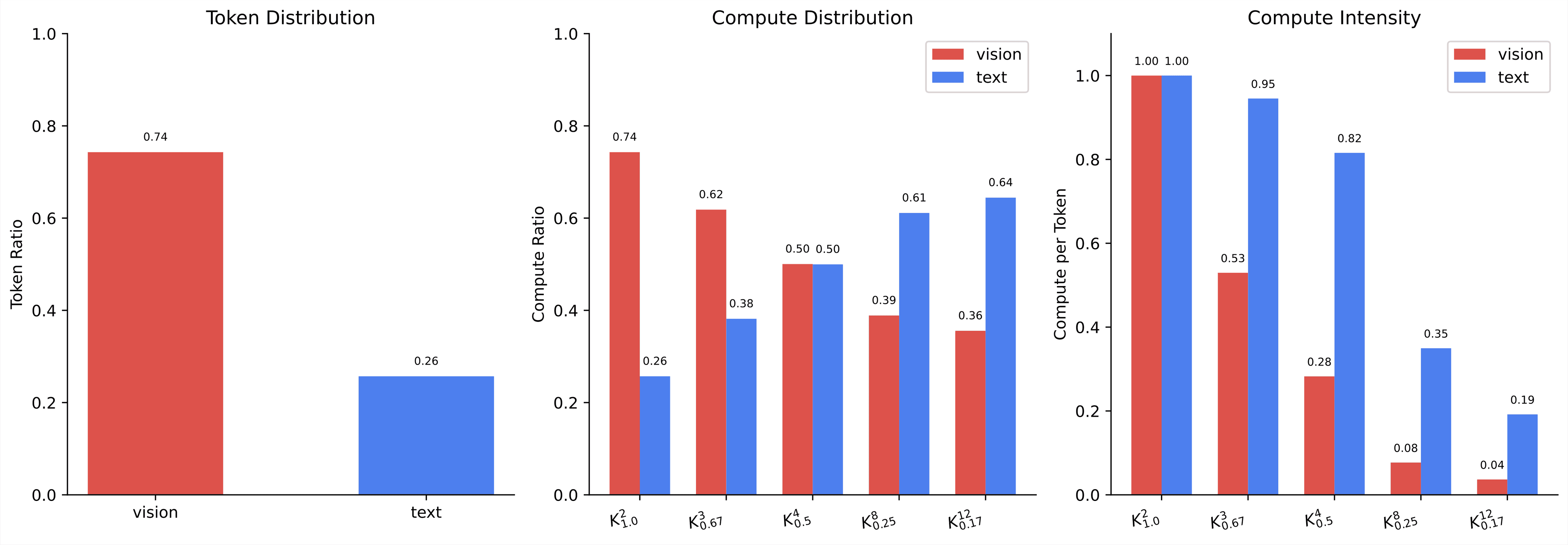
In dense configurations, vision consumes 74% of MoE compute (matching its token share). With null experts, the model routes vision tokens to nulls far more aggressively than text – inverting the distribution. At high sparsity, text consumes 64% of compute despite being only 26% of tokens.

No explicit modality routing. Just load balancing over an expanded pool.

Token-Level Compute Maps

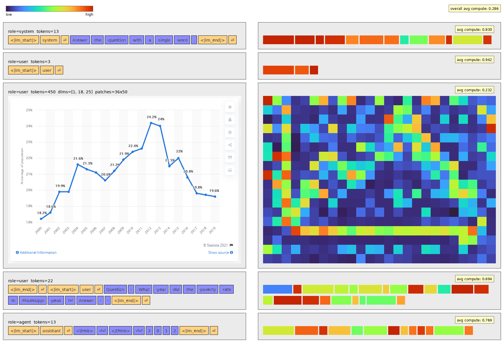
Bright = full computation, dark = null routing. The model allocates compute based on information content: salient image regions get more compute than background; dense text gets more than punctuation.

Task-Dependent Allocation

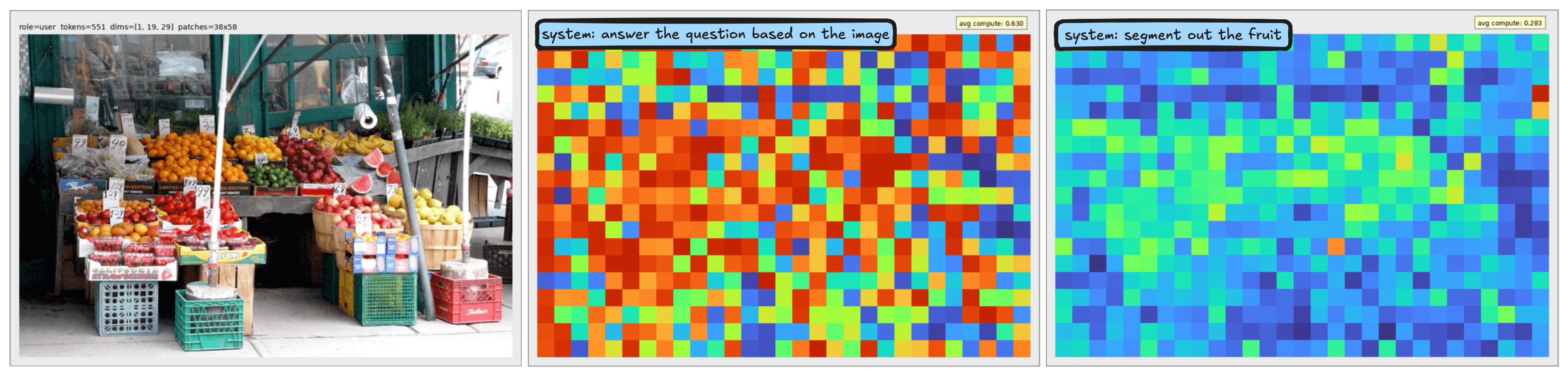
Same image, different prompts. Under a general QA prompt, compute distributes broadly. Under a targeted segmentation prompt, compute concentrates on task-relevant regions. The model learns that "relevant" is task-relative.

Takeaways

Weight and data sparsity are orthogonal efficiency axes. Standard MoE uses only weight sparsity. Composing both yields a better compute-efficiency frontier while preserving causality.

The model learns to allocate compute by information content: vision tokens route to nulls more than text, salient regions more than background, and allocation shifts based on task demands. All without explicit supervision.

@article{kilian2026composing,
  title={Improving MoE Compute Efficiency by Composing Weight and Data Sparsity},
  author={Kilian, Maciej and Mkrtchyan, Oleg and Zettlemoyer, Luke and Shrivastava, Akshat and Aghajanyan, Armen},
  year={2026}
}

Try Isaac Now

We believe in building in the open and empowering the community. You can start creating with Isaac today.

Read full paper

Try demo